Eddy-footprint Demo#
Author: Ludda Ludwig
Overview#
What is eddy-footprint?#
eddy-footprint is an open source python package for generating footprints for eddy covariance sites.
What is in this notebook?#
An example dataset of eddy covaraince fluxes. One day of footprints are generated using two types of footprint models. These footprints are made using the default domain extent (1000 meters) and resolution (5 meters). These footprints are made using parallelization at the rotation-interpolation step. These footprints are summed to create a daily composite image.
Footprints can be used internally as xarray objects for visualization or exported as netCDF files.
Examples are shown for plotting daily composite footprints.
Examples are shown for plotting a time-series of footprints as a facetgrid in xarray.
[1]:
import eddy_footprint as ef
import pandas as pd
import numpy as np
from matplotlib import pyplot as plt
import xarray as xr
Load the data#
[2]:
demo_datapath = "../data/demo.csv"
stable_datapath = "../data/stable_test.csv"
unstable_datapath = "../data/unstable_test.csv"
neutral_datapath = "../data/neutral_test.csv"
df_demo = pd.read_csv(
    demo_datapath,
    parse_dates=[1],
    na_values="NA",
    delimiter=" *, *",
    index_col=False,
    engine="python",
)
df_stable = pd.read_csv(
    stable_datapath,
    parse_dates=[1],
    na_values="NA",
    delimiter=" *, *",
    index_col=False,
    engine="python",
)
df_unstable = pd.read_csv(
    unstable_datapath,
    parse_dates=[1],
    na_values="NA",
    delimiter=" *, *",
    index_col=False,
    engine="python",
)
df_neutral = pd.read_csv(
    neutral_datapath,
    parse_dates=[1],
    na_values="NA",
    delimiter=" *, *",
    index_col=False,
    engine="python",
)
Create footprints using the Hsieh model#
[3]:
demo_foots_Hsieh = ef.calc_footprint(
    air_pressure=df_demo.air_pressure,
    air_temperature=df_demo.air_temperature,
    friction_velocity=df_demo.friction_velocity,
    wind_speed=df_demo.wind_speed,
    cross_wind_variance=df_demo.v_var,
    wind_direction=df_demo.wind_dir,
    monin_obukhov_length=df_demo.L,
    time=df_demo.datetime,
    instrument_height=2.53,
    roughness_length=0.0206,
    workers=-1,
    resolution=2,
)
Create footprints using the Kormann & Meixner model#
[4]:
demo_foots_KM = ef.calc_footprint(
    air_pressure=df_demo.air_pressure,
    air_temperature=df_demo.air_temperature,
    friction_velocity=df_demo.friction_velocity,
    wind_speed=df_demo.wind_speed,
    cross_wind_variance=df_demo.v_var,
    wind_direction=df_demo.wind_dir,
    monin_obukhov_length=df_demo.L,
    time=df_demo.datetime,
    instrument_height=2.53,
    roughness_length=0.0206,
    workers=-1,
    method="Kormann & Meixner",
    resolution=2,
)
Plot footprint climatologies#
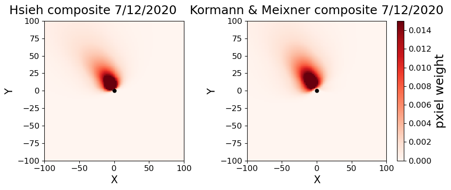
Stack of demo footprints (one day of half-hourly fluxes from July 12th 2020)
[5]:
stack_H = demo_foots_Hsieh.sum(dim="time")
stack_KM = demo_foots_KM.sum(dim="time")
Note that xarray objects have full matplotlib functionality.
[6]:
fig, axes = plt.subplots(nrows=1, ncols=2, figsize=(10, 4))

stack_H.plot(
    x="x", y="y", ax=axes[0], vmin=0, vmax=0.015, cmap="Reds", add_colorbar=False
)
axes[0].set_xlim([-100, 100])
axes[0].set_xlabel("X", fontsize=15)
axes[0].set_ylim([-100, 100])
axes[0].set_ylabel("Y", fontsize=15)
axes[0].set_title("Hsieh composite 7/12/2020", fontsize=18, pad=+10, x=0.35)
axes[0].plot(0, 0, marker=".", color="black", markersize=10)
axes[0].tick_params(labelsize=12)

im = stack_KM.plot(
    x="x", y="y", ax=axes[1], vmin=0, vmax=0.015, cmap="Reds", add_colorbar=False
)
axes[1].set_xlim([-100, 100])
axes[1].set_xlabel("X", fontsize=15)
axes[1].set_ylim([-100, 100])
axes[1].set_ylabel("Y", fontsize=15)
axes[1].set_title("Kormann & Meixner composite 7/12/2020", fontsize=18, pad=+10)
axes[1].plot(0, 0, marker=".", color="black", markersize=10)
axes[1].tick_params(labelsize=12)
cb = plt.colorbar(im, orientation="vertical", pad=0.05)
cb.set_label(label="pxiel weight", fontsize=18)
cb.ax.tick_params(labelsize=12)
axes[0].set_aspect("equal")
axes[1].set_aspect("equal")
fig.tight_layout()
fig.subplots_adjust(wspace=0)
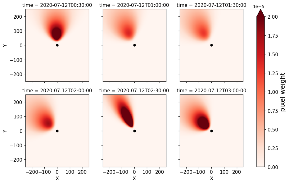
Plot multiple footprints in the timeseries as a facetgrid
Slice a subset to plot
Make facetgrid
Add marker for the tower location at 0,0
[7]:
time_slice = demo_foots_Hsieh.isel(time=slice(0, 6, 1))
print(time_slice.coords)
fig_facet = time_slice.plot(
    x="x",
    y="y",
    col="time",
    col_wrap=3,
    cmap="Reds",
    vmax=2e-5,
    cbar_kwargs={"label": "pixel weight"},
)
fig_facet.map(lambda: plt.plot(0, 0, marker=".", color="black", markersize=10))
fig_facet.cbar.ax.tick_params(labelsize=11)
fig_facet.cbar.set_label(fontsize=15, label="pixel weight")
fig_facet.set_titles(fontsize=11)
fig_facet.set_xlabels("X", fontsize=12)
fig_facet.set_ylabels("Y", fontsize=12)
fig_facet.set_ticks(fontsize=11)
plt.xlim(-250, 250)
plt.ylim(-250, 250)
Coordinates:
  * time     (time) datetime64[ns] 2020-07-12T00:30:00 ... 2020-07-12T03:00:00
  * x        (x) float64 -1e+03 -998.0 -996.0 -994.0 ... 994.0 996.0 998.0 1e+03
  * y        (y) float64 -1e+03 -998.0 -996.0 -994.0 ... 994.0 996.0 998.0 1e+03
[7]:
(-250.0, 250.0)
Export xarray dataset as netcdf#
[8]:
netcdf_path = "../data/demo_footprints_Hsieh.nc"
demo_foots_Hsieh.to_netcdf(netcdf_path)
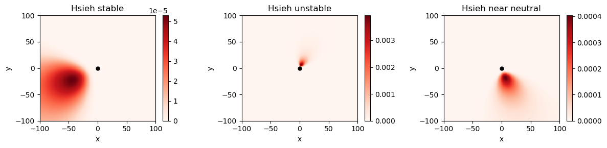
Explore footprints from different atmospheric conditions#
[9]:
stable_foots_Hsieh = ef.calc_footprint(
    air_pressure=df_stable.air_pressure,
    air_temperature=df_stable.air_temperature,
    friction_velocity=df_stable.friction_velocity,
    wind_speed=df_stable.wind_speed,
    cross_wind_variance=df_stable.v_var,
    wind_direction=df_stable.wind_dir,
    monin_obukhov_length=df_stable.L,
    time=df_stable.datetime,
    instrument_height=2.53,
    roughness_length=0.0206,
    workers=-1,
    resolution=1,
)
unstable_foots_Hsieh = ef.calc_footprint(
    air_pressure=df_unstable.air_pressure,
    air_temperature=df_unstable.air_temperature,
    friction_velocity=df_unstable.friction_velocity,
    wind_speed=df_unstable.wind_speed,
    cross_wind_variance=df_unstable.v_var,
    wind_direction=df_unstable.wind_dir,
    monin_obukhov_length=df_unstable.L,
    time=df_unstable.datetime,
    instrument_height=2.53,
    roughness_length=0.0206,
    workers=-1,
    resolution=1,
)
neutral_foots_Hsieh = ef.calc_footprint(
    air_pressure=df_neutral.air_pressure,
    air_temperature=df_neutral.air_temperature,
    friction_velocity=df_neutral.friction_velocity,
    wind_speed=df_neutral.wind_speed,
    cross_wind_variance=df_neutral.v_var,
    wind_direction=df_neutral.wind_dir,
    monin_obukhov_length=df_neutral.L,
    time=df_neutral.datetime,
    instrument_height=2.53,
    roughness_length=0.0206,
    workers=-1,
    resolution=1,
)
Create footprints using the Kormann & Meixner model for the two test regimes
[10]:
stable_foots_KM = ef.calc_footprint(
    air_pressure=df_stable.air_pressure,
    air_temperature=df_stable.air_temperature,
    friction_velocity=df_stable.friction_velocity,
    wind_speed=df_stable.wind_speed,
    cross_wind_variance=df_stable.v_var,
    wind_direction=df_stable.wind_dir,
    monin_obukhov_length=df_stable.L,
    time=df_stable.datetime,
    instrument_height=2.53,
    roughness_length=0.0206,
    workers=-1,
    method="Kormann & Meixner",
    resolution=1,
)
unstable_foots_KM = ef.calc_footprint(
    air_pressure=df_unstable.air_pressure,
    air_temperature=df_unstable.air_temperature,
    friction_velocity=df_unstable.friction_velocity,
    wind_speed=df_unstable.wind_speed,
    cross_wind_variance=df_unstable.v_var,
    wind_direction=df_unstable.wind_dir,
    monin_obukhov_length=df_unstable.L,
    time=df_unstable.datetime,
    instrument_height=2.53,
    roughness_length=0.0206,
    workers=-1,
    method="Kormann & Meixner",
    resolution=1,
)
Plot the footprints from different atmospheric conditions:
[11]:
fig, axes = plt.subplots(nrows=1, ncols=3, figsize=(12, 3))

stable_foots_Hsieh.isel(time=1).plot(x="x", y="y", ax=axes[0], cmap="Reds")
axes[0].set_xlim([-100, 100])
axes[0].set_ylim([-100, 100])
axes[0].plot(0, 0, marker=".", color="black", markersize=10)
axes[0].set_title("Hsieh stable")

unstable_foots_Hsieh.isel(time=1).plot(x="x", y="y", ax=axes[1], cmap="Reds")
axes[1].set_xlim([-100, 100])
axes[1].set_ylim([-100, 100])
axes[1].plot(0, 0, marker=".", color="black", markersize=10)
axes[1].set_title("Hsieh unstable")

neutral_foots_Hsieh.isel(time=1).plot(x="x", y="y", ax=axes[2], cmap="Reds")
axes[2].set_xlim([-100, 100])
axes[2].set_ylim([-100, 100])
axes[2].plot(0, 0, marker=".", color="black", markersize=10)
axes[2].set_title("Hsieh near neutral")

fig.tight_layout()
[ ]: